
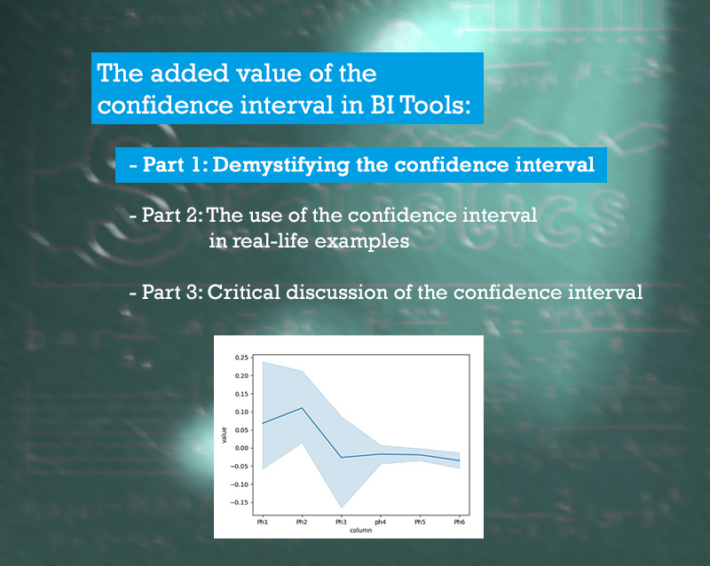
Part 1 – Demystifying the confidence interval
Introduction
I’ve always been intrigued by a statistic metric in the human sciences called the confidence interval. In summary, the confidence interval is defined as a statistical measure of reliability. It says something about your statistical outcome by comparing it with all potential results given the data on which the statistical analysis is based on. In other words, the metric can add value to your analytical endeavors because it gives in a certain way access to nothing more than the… multiverse. In this blog I want to explain why this is the case and furthermore, I want to show you, the data professional, how to harness the power of the confidence interval in the mainstream BI tools.
There is a lot to say about the confidence interval. Because of this I’ve decided to split the total article up in 3 separate blogposts: (a) the first one covers the definition of the confidence interval without relying on complex mathematical concepts and formulas; (b) in the second part you will master the confidence interval by learning how it used in real-life examples in Power BI; (c) I will conclude the 3 part set with a critical view of the added value of the confidence interval in your analysis. Let’s dive in.
The confidence interval explained in l(h)aymen’s terms

Let’s start with an example: your boss has ordered you to find the needle in a haystack. In statistics, this needle is our parameter of interest. You know the needle is in the haystack (= all data or population) but you don’t know it’s exact location. You don’t want to use all resources to search for the needle, so what you do is, you grab a pile of the hay where you know it’s most likely to be there (= sample). Now it’s time for you to present your findings to your boss.

Before I continue with this exciting story, I want to have a short detour to focus on why it is practically impossible to find the needle or the true value of a certain parameter. This relates to the concept “population”. The population is nothing more than an abstract idea. This collection of all observations is not directly accessible because it holds all potential outcomes. This includes all the results that could have happened but did not happen. Think of it like we live in a universe that’s part of an infinite number of parallel universes, each for every possible outcome and they exist all at once (the multiverse). For instance, let’s say you have all sales data for measuring the average amount of sales per dealer. In the context of the multiverse, this is still a sample, because on the population level you will always be short in having all the data to measure the true average amount of sales per dealer. Why might you ask? Because in your universe a dealer may have just missed a sale while in a very slightly different parallel universe that same dealer could have nailed it. All the different parallel universes are inaccessible, unless… you are Dr. Strange. Also, we don’t live in a science fiction movie. However, the theory of parallel universes points out to an important question: how can we consider all possibilities from one sample? Answer: with the confidence interval. The power of the mathematical model underlying the confidence interval takes all and every possible outcome into account given the sample that is used. I find this intriguing because by using the confidence interval, we do have in some sense access to the multiverse.
Continuing with the story: you grabbed a pile of hay and now it’s time for you to present your findings to your boss. From the sampled hay, you handover another pile. Dependent on how big this pile is, 2 scenarios are possible:
- Scenario 1: big pile of hay (= high accuracy or a high confidence level).
- If you use a bigger pile, you will have higher confidence that your stack has the needle. But your boss won’t be happy to receive a ton of hay to find a needle. You get accuracy with high confidence level, but you lose precision.
- Scenario 2: small pile of hay (= low accuracy or a low confidence level)
- if you use a smaller pile of hay, it will be easy for you to carry it and hand it over to your boss, but you won’t have that high confidence of being successful in your mission. You get precision but you lose accuracy with low confidence.
In a business context, scenario 2 is the preferred scenario because it’s a practical solution. In real life, instead of presenting a small pile of hay to your boss, you report a sample estimate of the population value to help decision making. It’s common practice to present a single number as a sample estimate. In statistics this is called a point estimate. An estimate could be in the form of a proportion, mean, percentile, correlation, coefficient… (to name a few). Whatever form it takes, if we go back to the haystack example, you are actually presenting one single straw: the best point estimate for the needle. It’s praised with high precision but flawed with low accuracy. Let me explain this graphically.
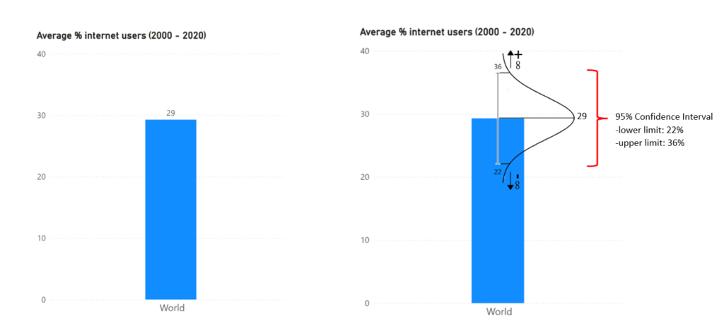
The point estimate in the both bar graphs above show the 20-year average proportion of internet users worldwide, which is equal to 29%. This value is the result of averaging 20 datapoints (a datapoint = % internet users in a year between 2000 – 2020). Each datapoint is the result of an unimaginable number of influences. We can assume that it wouldn’t have taken much to change one of those influencing factors and thus the final value of a datapoint. If we want to be as accurate as possible, every possible change, even an infinite minor one, should be presented in our analysis. One single number doesn’t cut it. So, if we want to be 100% accurate, we need to take the multiverse into account which means we end up with an infinite list of possibilities. Not practical to say the least, so not favored by the business. We need a trade-off. Thankfully, mathematical models tell us that the parallel universes can be ranked in a normal distribution symmetrically centered around the point estimate. The normal distribution is shown in the right bar graph. Somewhere in this normal distribution resides the population value aka the needle. We cannot say where precise, but the normal distribution makes it practically possible to ballpark it. This can be done by selecting a range in the normal distribution and deferring how certain we can be that the population value is somewhere in this area. This range is called the confidence interval.
The confidence interval is defined by a lower limit and an upper limit. With 100% accuracy and 0% precision the limits would be endless (-∞; +∞). It covers all the possible results. The exact opposite, 0% accuracy and 100% precision, is the point estimate. A narrower confidence interval is a way to deal with the trade-off between accuracy and precision. In the right bar graph, I’ve chosen for a range that covers 95% of the normal distribution. This results in a confidence interval with a lower limit of 22% average internet users and an upper limit of 36% average internet users. The conclusion is that we can be 95% confident that the true value of yearly average % internet users in the period of 2000 – 2020 will be between 22% and 36%. The amount of confidence, which I also referred to as accuracy, is called the confidence level. The difference between the limit value and the point estimate is the margin of error. In this example the |margin of error| is equal to 7% (limit value – 29%). Ideally, you want the margin of error as small as possible.
Conclusion
The confidence interval is not an easy concept to grasp if it is compared to other statistics such as the correlation or standard deviation. Hopefully, with this first part, I’ve made it easier to understand. As you noticed, there is no need for a mathematical background to use the confidence interval in BI. The most important aspects you need to understand are:
- The confidence interval is a range with a lower limit and upper limit, covering a proportion (%) of all possibilities.
- The confidence level defines the interval and is the % of all possibilities taken into account in the interval. It tells us how confident (0% – 100%) we are that the true value lies in the interval
- The considered possibilities are ranked in a normal distribution symmetrically centered around the point estimate
- The margin of error is the difference between the limit value and the point estimate
In the second part, the confidence interval will be used in real-life BI examples. The goal is get you on board with using and explaining the confidence interval in your own BI analysis.